Worked examples

Every figure on this page is generated by examples/generate_docs_figures.py against itis-sumo's real public API — a real (unmocked) Dakota GP fit, the real LHS sampler, the real Sobol' pipeline — on small analytical problems chosen because the right answer is known in closed form. Regenerate them yourself with:

uv run --group docs python examples/generate_docs_figures.py

For the real-application examples referenced in the roadmap below (NIH in-silico model, and datasets from Paria, Giuliana, Luisa), see the Provenance / Porting page and the corresponding Project House tasks — those write-ups will be added here as they land.

1. A GP surrogate fit, with its own uncertainty

Theory: how Gaussian Processes work covers the math; here is the actual shape of it. Nine training points sampled from \(f(x) = \sin(x)\) on \([0, 2\pi]\), fit through itis-sumo's real evaluate_sumo, evaluated on a dense grid:

from itis_sumo.evaluate.funs_evaluate import evaluate_sumo

# x_train: 9 points, y_train = sin(x_train), written as a Dakota training file
result = evaluate_sumo(run_dir, train_file, eval_file, ["x"], "y")
y_hat = result["y_hat"]        # posterior mean, μ(x)
y_std = result["y_std_hat"]    # posterior std, σ(x) — V8df in SPEC.md

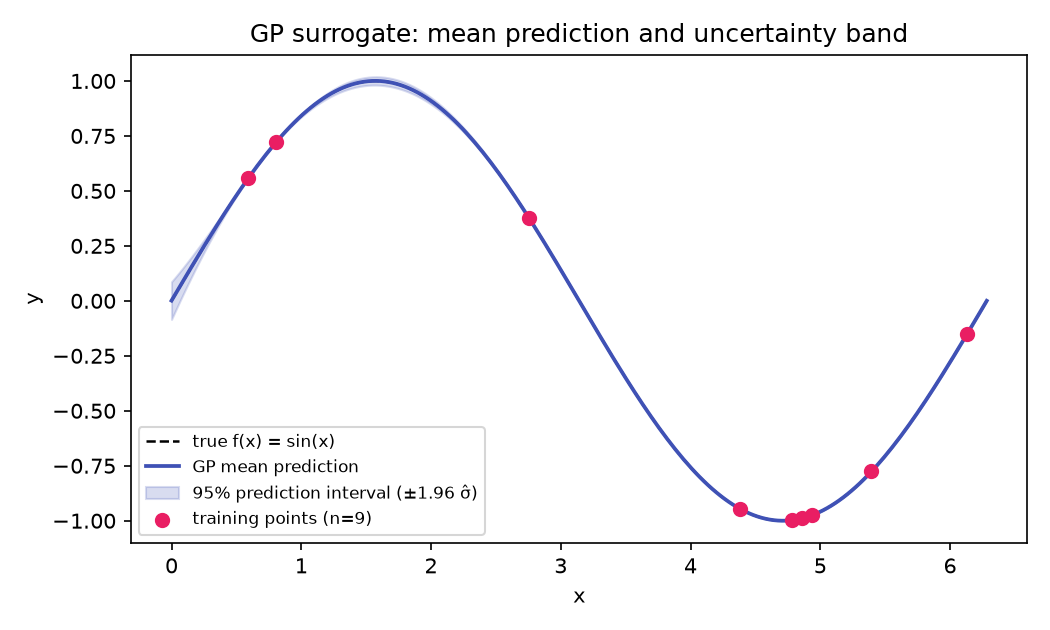
Notice the band pinches to (near) zero width right at each training point and widens between them — that's the posterior variance formula \(\sigma^2(\mathbf{x}_*) = k(\mathbf{x}_*,\mathbf{x}_*) - \mathbf{k}_*^\top (K+\sigma_n^2 I)^{-1}\mathbf{k}_*\) from the GP theory page made visible: query points near training data have large kernel similarity to something already observed (small subtracted term, small variance); query points far from all training data don't (large variance). This is the same mechanism the test suite checks numerically in test_variance_near_zero_at_training_points_grows_away.

2. Why Latin Hypercube sampling, not plain random

Sampling theory argues that training-point placement matters as much as training-point count. 25 points each, drawn two ways, using itis-sumo's real lhs():

from itis_sumo.sampling.lhs import lhs

lhs_pts = lhs(2, 25, method="maximin", seed=42)   # stratified: one draw per 1/25 bin, per axis
rand_pts = rng.uniform(0.0, 1.0, size=(25, 2))     # i.i.d. uniform — no stratification guarantee

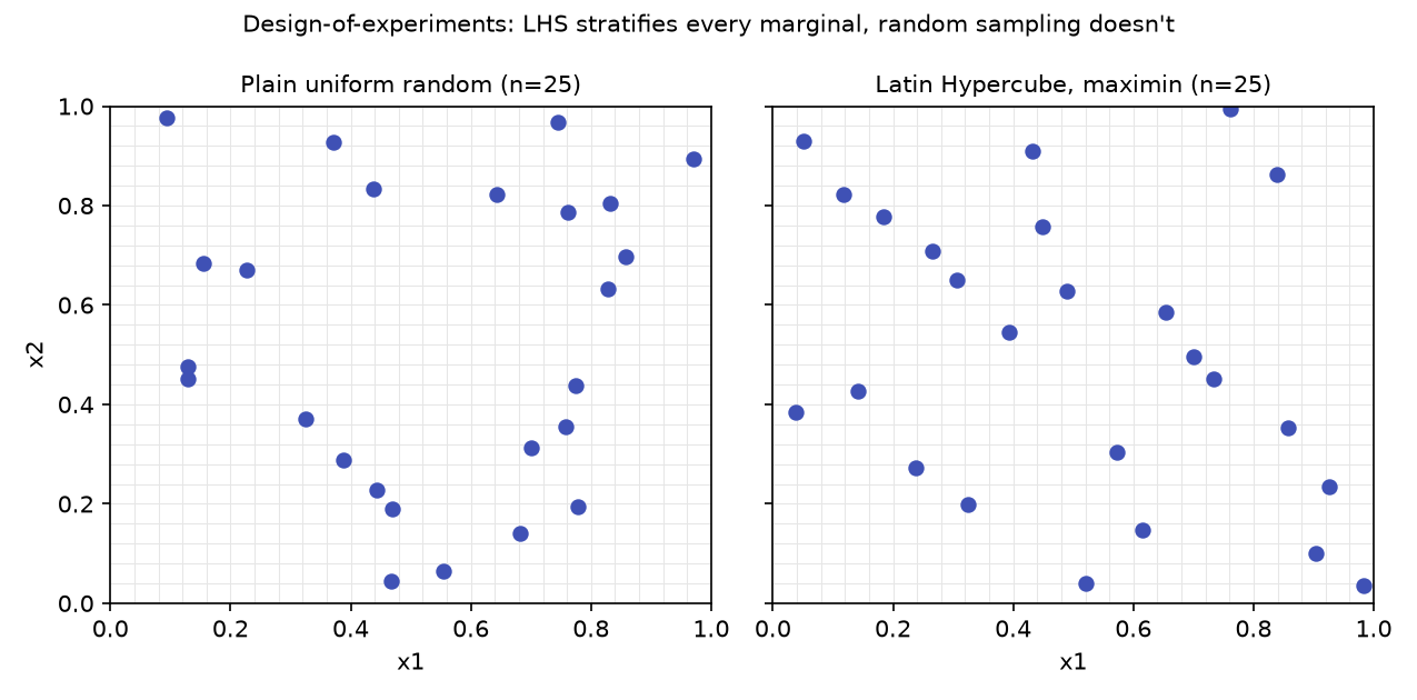
The random draw (left) visibly clusters in some regions and leaves gaps in others — pure chance, but chance that wastes training budget where two points land close together and tell the surrogate almost nothing it didn't already know. LHS (right) guarantees each of the 25 equal-width bins along both x1 and x2 contains exactly one point — every training run is guaranteed even 1D marginal coverage, which is what the seeded-RNG invariant V3er in SPEC.md exists to make reproducible.

3. Sensitivity analysis on a surrogate: does it recover the right physics?

The Ishigami function is the standard analytical test case for sensitivity methods because its Sobol' indices are known in closed form — see Reference → Sensitivity (Sobol) & UQ for the derivation. This is not the pure-math validation already covered there (which bypasses the surrogate entirely) — this trains a real GP on 300 noisy-free samples of the Ishigami function and runs the full evaluate_sobol_indices pipeline, surrogate included:

sobol = evaluate_sobol_indices(
    run_dir, train_file, ["x1", "x2", "x3"], "y1", distributions, preprocessor, seed=42
)["sobol"]

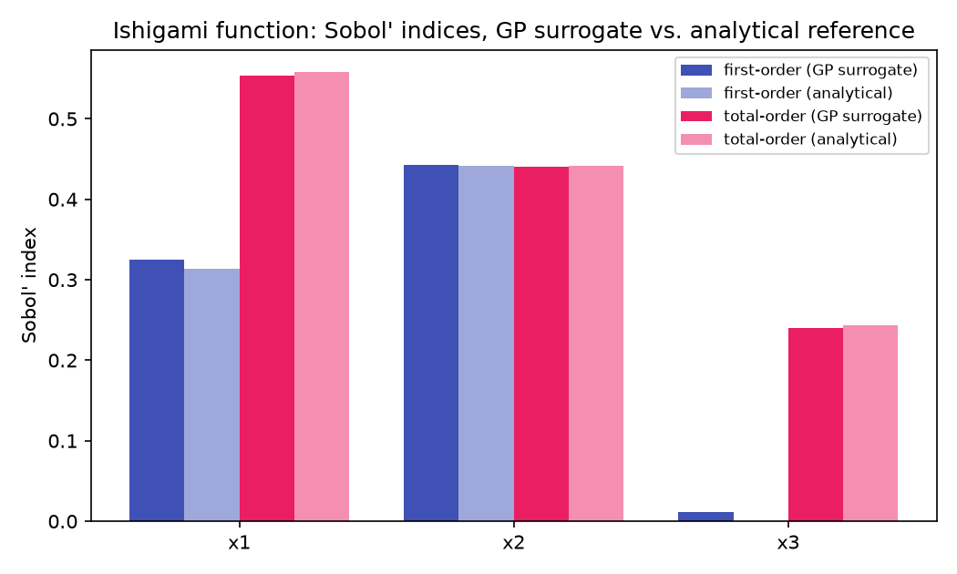
The GP-surrogate-derived indices (dark bars) track the analytical reference (light bars) closely for all three variables and both index orders — including correctly recovering that x3 has zero first-order effect despite having a large total-order effect (\(S_3 \approx 0\), \(S_{T3} \approx 0.244\)), which is only possible because of Ishigami's x1–x3 interaction term. A surrogate that got the interaction structure wrong would show up here as a x3 total-order bar collapsing toward its (near-zero) first-order bar. This is the sensitivity-analysis analogue of the GP-fit sanity check above: trust in the downstream analysis is only as good as the surrogate it's built on, and this is what it looks like when that trust is earned rather than assumed.

Real-application examples (in progress)

The three worked examples above are analytical sanity checks — closed-form answers, no ambiguity about whether the surrogate got it "right." The next phase of validation work is running itis-sumo against real, previously unseen application data, where there's no closed-form answer to check against and the real question is whether the surrogate + UQ + sensitivity pipeline gives trustworthy, decision-useful answers on a genuine research problem. Four such applications are tracked as Project House tasks:

1. NIH in-silico model — prioritized first.
2. Real bioelectronic/simulation datasets contributed by Paria, Giuliana, and Luisa.

Each will be written up here as a dedicated example page once the underlying validation work lands.