TI Analysis

Summary

Classic TI: Based on the selected model and target, the surrogate-modeling-based optimizer (SuMo) systematically explores the solution space to identify optimal configurations considering three key metrics:

• strength: the median of the TI modulation envelope magnitude (T_max) within the target
• selectivity: the signal-to-noise ratio of TI exposure — squared ratio of the RMS of T_max in the target to the RMS of T_max in the off-target brain: (RMS_target / RMS_off-target)²
• collateral: the fraction of the non-target brain volume with T_max exceeding the p-th isopercentile of T_max in the target or the brain (p is user-configurable)

These metrics are also central to the visualization and included in the downloadable report.

By combining Gaussian process modeling with a multi-objective genetic algorithm, the SuMo optimizer provides a diverse set of Pareto-optimal solutions. This allows users to easily navigate trade-offs like selectivity versus intensity, making informed choices with regard to conflicting TI exposure criteria. As of TIP V5.2, The optimizer launches multiple independent searches, seeds, in parallel, each of which explores the electrode search space from a different starting point. The individual Pareto fronts are merged by means of non-dominated sorting into a single combined front that provides a denser Pareto front with wider coverage, richer configurations, and overall superior solutions, as quantified by the hypervolume indicator. Furthermore, instead of always running to a maximum iteration count, each seed now monitors for convergence after every iteration and stops automatically once meaningful improvement ceases. Users can choose between low, medium, and high precision modes, whereby low provides a quick first look after about 5 minutes and high delivers the most exhaustive Pareto-front coverage, requiring 30 minutes to one hour.

Starting from a thus optimized, or from a user-defined TIS configuration, the resulting exposure can be studied and if desired, the configuration (electrode locations, current magnitudes) can be interactively refined. For that purpose, TI and high-frequency exposure distributions are dynamically visualized on top of medical image data, and key exposure metrics as well as plots are shown.

Once promising exposure conditions have been identified, the associated visualizations and metrics can be added to an automatically generated, downloadable report.

Multi-channel and phase-modulation TI: For multi-channel and phase-modulation TI, the offered functionality is slightly different. Additional or alternative settings are presented, reflecting the obvious differences in relevant stimulation parameters (e.g., targeted modulation shape, number of channels and channel frequencies). Also the definition of the Quantities-of-Interest necessarily differs (see here). Finally, the vast parameter space of multi-channel and phase-modulation TI currently prohibits systematic optimization, such that only user-specified configurations can be analyzed.

---

TIP Lite

In TIP Lite, this service is available in a reduced form. The table below summarizes what is and is not available compared to full TIP:

Feature	TIP Lite	Full TIP
Classic TI mode	✓	✓
SuMo optimizer and Pareto-optimal configuration table	✓	✓
Exposure visualization (2D/3D slices, waveforms, iso-surface)	Full	Full
Available anatomical models	MIDA (anisotropic) and Mouse	All precomputed models + personalized
Multi-channel TI and phase-modulation TI modes	—	✓
Export to S4L (.cache) and Exposure Analysis	—	✓
Report generation	—	✓

TIP Lite is designed for users new to TI or with basic planning needs. Upgrade to full TIP to access optimization, advanced analysis, and reporting capabilities.

---

Analysis

Classic TI

The Settings section at the top allows you to configure essential optimization parameters:

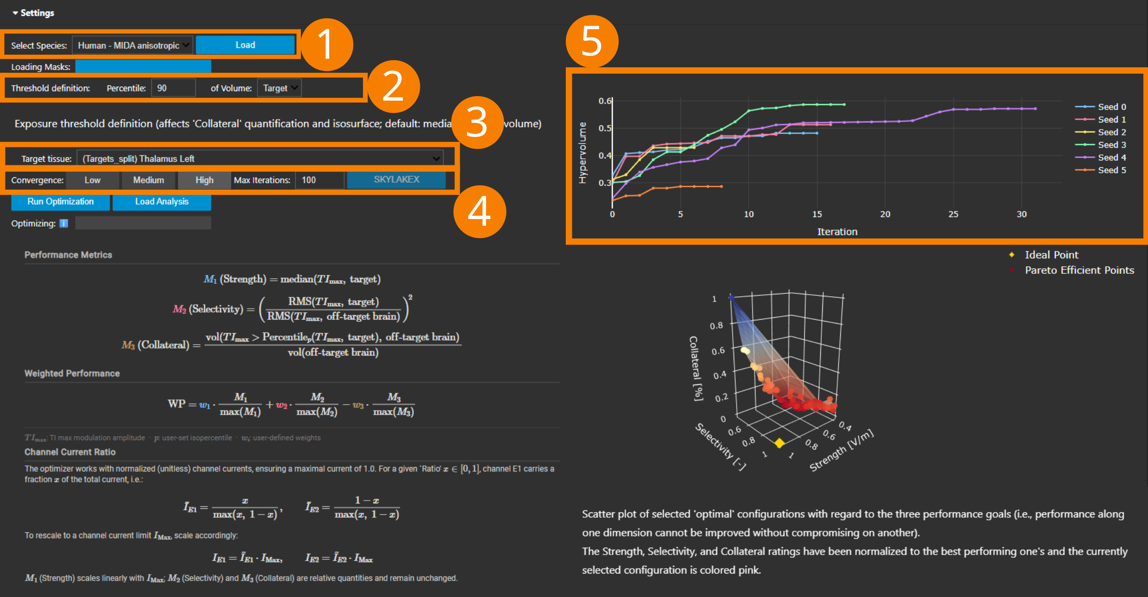
1. Select Species

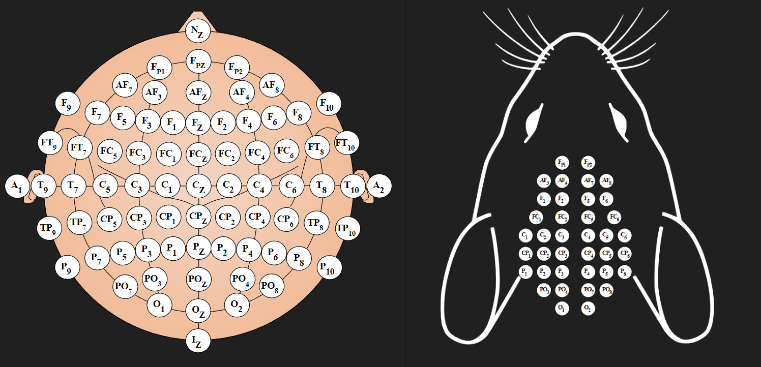
   Choose the anatomical model type (human or mouse) from the drop-down menu. Each species comes with pre-configured standard electrode locations appropriate for that anatomy. Additional species options are planned for future releases.

2. Threshold definition

Define how stimulation thresholds should be calculated by selecting either the entire brain or only the target region as your reference, and specify the appropriate isopercentile level for precise threshold determination.

3. Target tissue

Specify the exact brain structure you wish to target with TI stimulation. This selection serves as the foundation for calculating and optimizing all exposure quality metrics.

4. Convergence

Select from low, medium or high convergence requirement. The low setting is meant for fast exploration of different setting parameter choices. This comes at the cost of HV score. The medium setting gives a balance between optimization speed and performance, suitable for situations where time is limited but the quality of the pareto front should also be higher. The high constraint yields the best HV score. This should be used when the other parameters are fixed and a rich pareto front is needed to support your electrode setup decision.

Max Iterations can be increased in case convergance isn't reached even after the default 100 iterations. For most cases 100 iterations is sufficient.

The last box in this section indicates the OpenBLAS kernel currently in use. This is not meant for interaction. It only shows which kernel is available on the infrastructure the service is running on. On modern AVX-512 CPUs this defaults to the SKYLAKEX kernel. Since the kernel affects the optimization results, we added the following safety precatution: If the service detects that the kernel changed from the last time the service was used, this box will turn red. If this happens to you, please get in touch with us.

5. Seed Convergence

This plot show you the convergence behaviour of all the different seeds while the optimization is running. This allows you to see the progress and estimate approximately how long the process might still run.

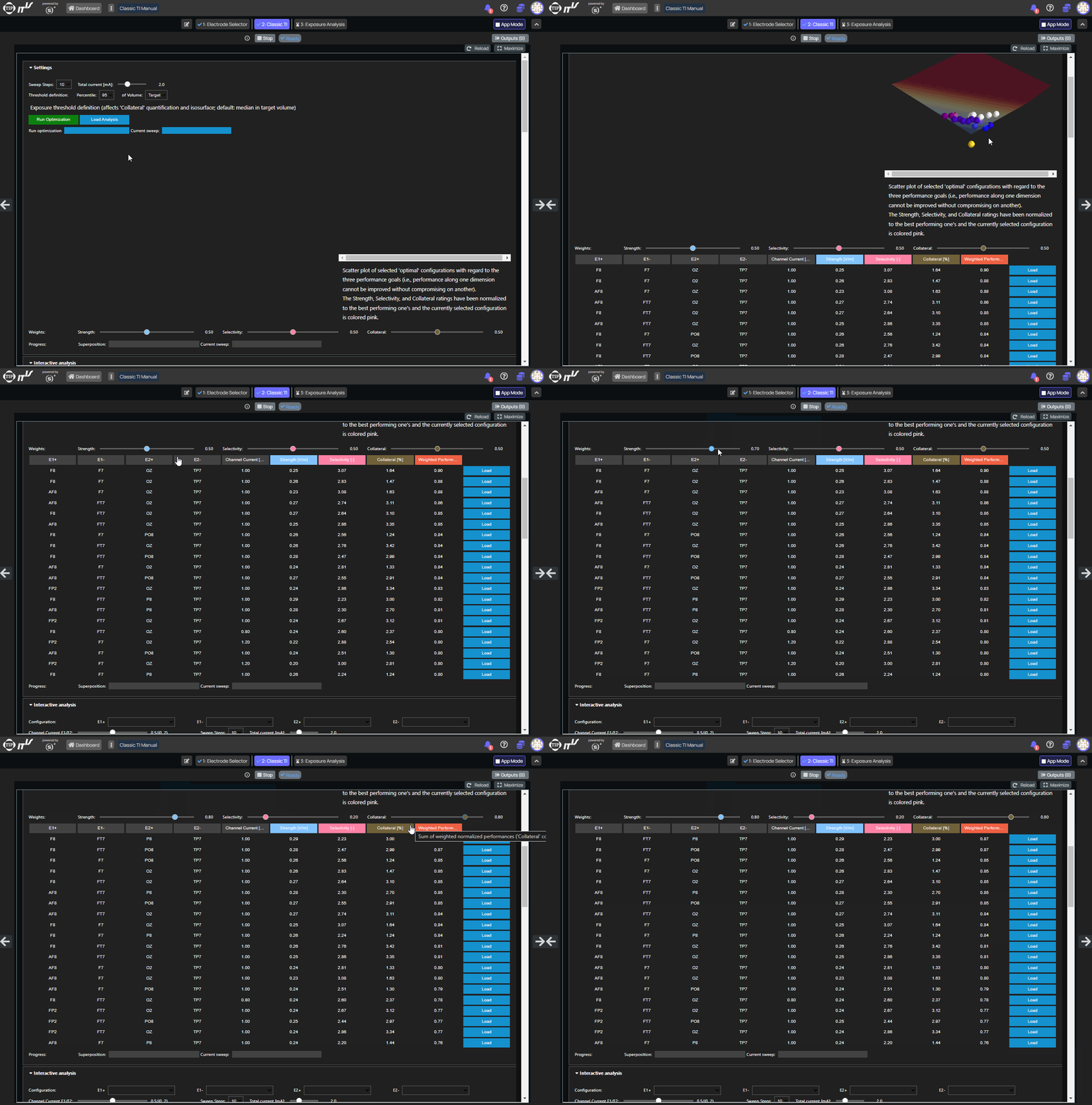
After running the optimization with the SuMo engine and loading the analysis, you'll see a comprehensive view of the results. The interactive table displays all Pareto-optimal electrode configurations ranked by their performance across three key metrics: Strength, Selectivity, and Collateral. Below this table, detailed visualization panels let you examine field distributions in both 2D and 3D views, along with comprehensive waveform analysis.

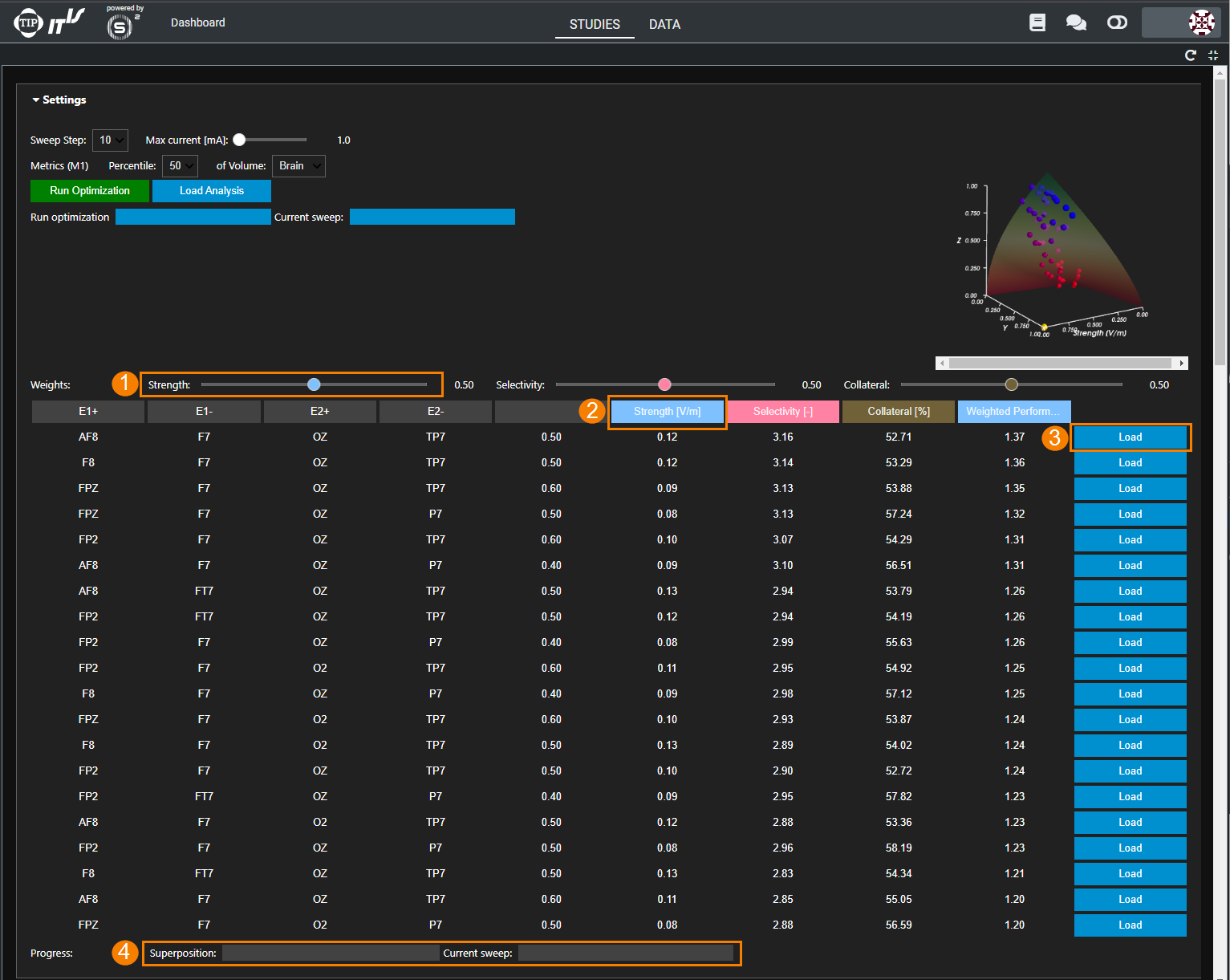
Use the intuitive weighting sliders at the top (1.) to prioritize metrics according to your research objectives. Adjust the relative importance of Strength, Selectivity, and Collateral stimulation, and the table automatically sorts configurations by the resulting composite score (displayed in the rightmost column). You can also sort by any individual metric by clicking directly on the column header (2.).

The interactive 3D scatter plot provides a visual representation of the Pareto front, allowing you to quickly understand the trade-offs between different performance metrics and identify the most promising Pareto-optimal solutions for your specific application.

When you've identified a promising configuration, click the Load button (3.) to examine it in detail. The system performs a targeted sweep across channel weights to prepare the visualization, making subsequent exploration more responsive. A progress indicator (4.) shows the status of this optimization process.

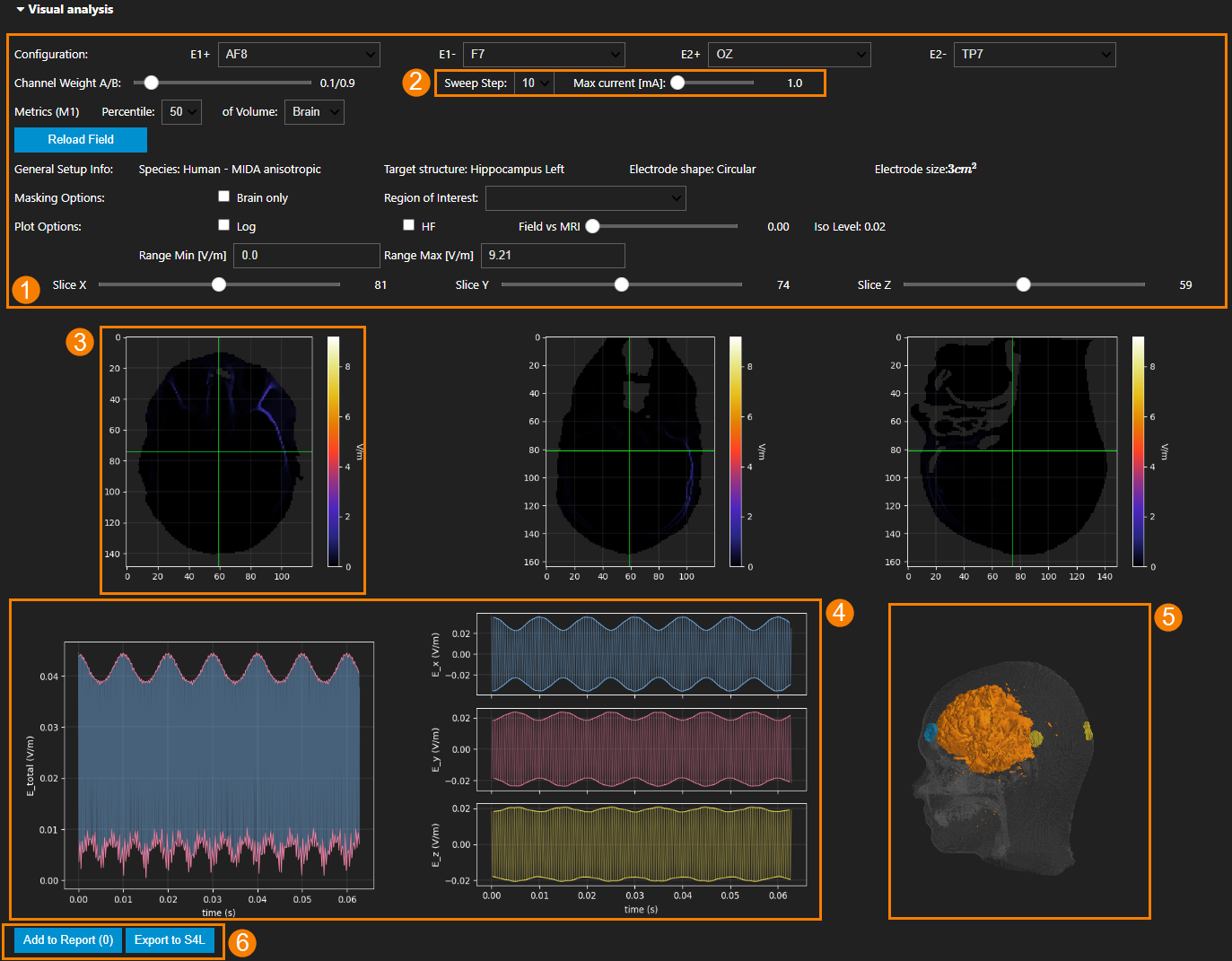
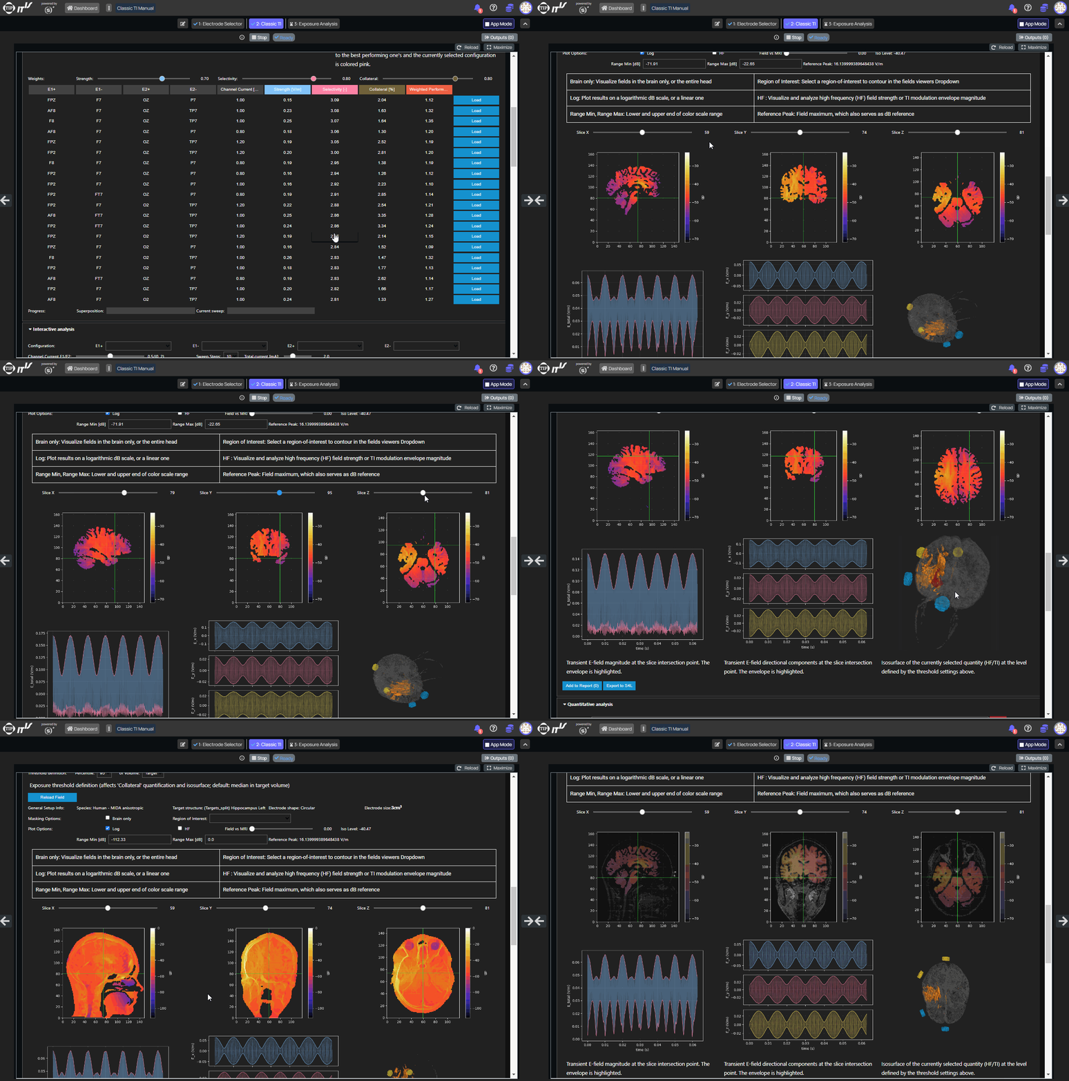
Once that sweep is complete, all the viewers in the lower half of the screen are updated. Now you can visually inspect the exposure scenario:

1. Main Controls

   This comprehensive control panel provides all visualization settings:

   • Configuration: Adjust electrode positions freely and update the field visualization by clicking the Reload Field button.
   • Channel Current A/B: Fine-tune the relative contribution of each channel using the intuitive slider control.
   • Performance Metrics: Customize the metrics calculation by selecting the appropriate volume and isopercentile level.
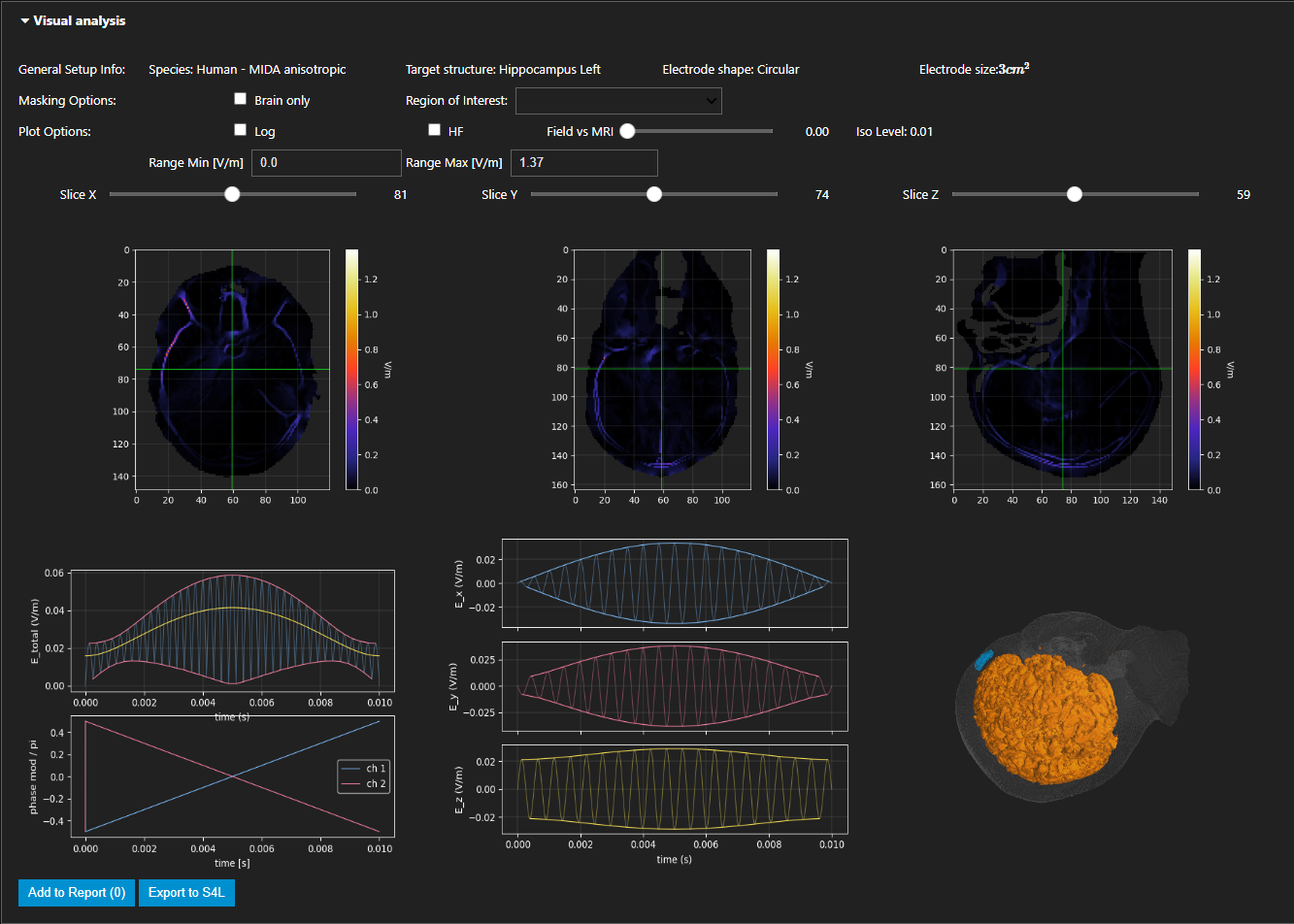
   • Masking Options: Focus on specific anatomical areas by toggling between whole head and brain-only views. Use the Region of Interest dropdown to highlight specific brain regions for detailed analysis. Select None to return to the default view without highlighting.
   • Plot Options: Switch between Log and dB scales, or toggle between high frequency (HF) and temporal interference (TI) field visualizations. Adjust the balance between field visualization and underlying MRI data using the Field vs MRI opacity slider.
   • Value Range: Fine-tune the visualization range by modifying Range Min and Range Max values for enhanced detail in areas of interest.
   • Slice Navigation: Position the orthogonal slice planes precisely using the Slice X, Slice Y, and Slice Z sliders.

2. Advanced Parameter

   Unlike other controls that update the visualization instantly, this parameters require additional computation when changed:

   • Sweep Step: Controls the resolution of the channel current ratio sweep, with higher values providing more detailed analysis.

   After adjusting these parameters, click the Reload Field button to recalculate the field distributions and update all visualizations.

3. Slice Viewers

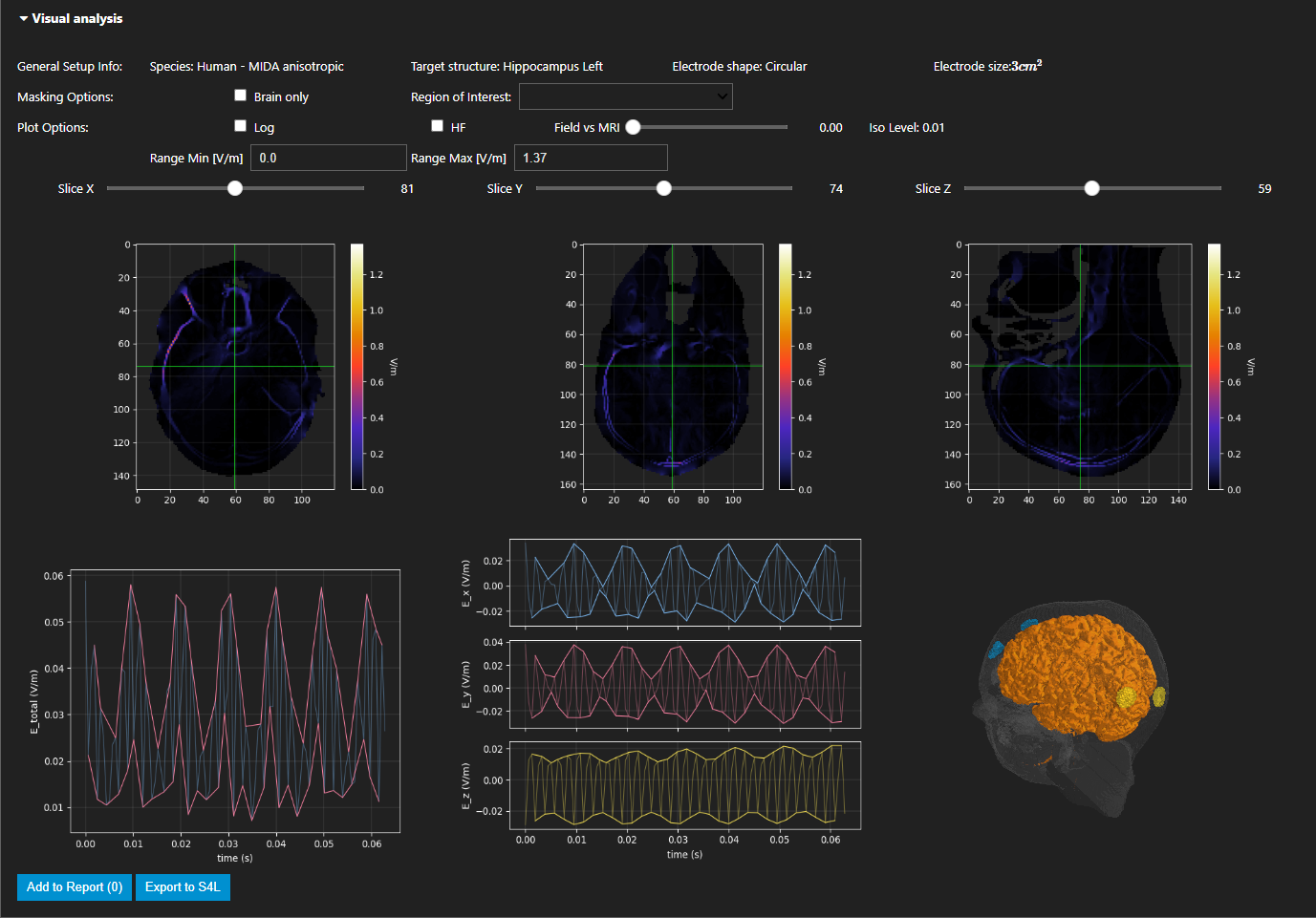
   The three orthogonal slice views display field distributions overlaid on the original MRI data. Interactive crosshairs indicate the intersections between slice planes, providing spatial context. Navigate through the volume easily by either:

   • Using the dedicated sliders (Slice X, Slice Y, and Slice Z)
   • Directly clicking on any location within a slice view (which automatically repositions all crosshairs)

4. E-Field Envelope

   These graphs show the transient E-Field at the location of the crosshair in slice views (3.). The absolute field magnitude and the x, y, and z components are displayed. The plots show both the high-frequency transient E-field, as well as the low-frequency TI envelope.

5. Iso-Surface View

   An interactive 3D model of the current setup: The electrode pair locations are shown in yellow and blue, the target in red, and the iso-surface in orange. The iso-surface visualizes all voxels with value equal to the strength metric reached within the target.

6. Export Buttons

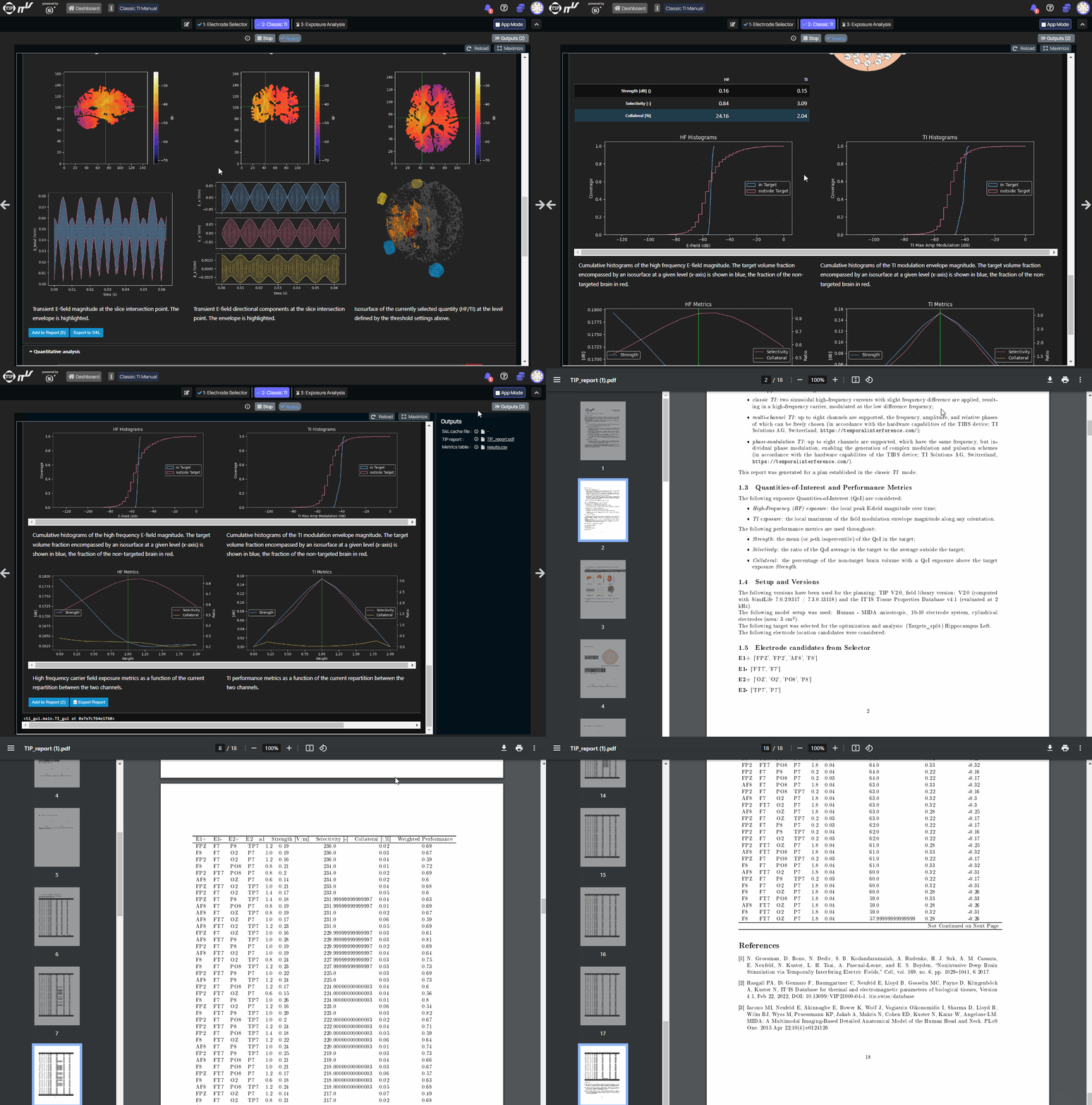
   • Add to Report allows addition of the six viewing elements to the PDF report (according to the currently selected slicing positions and viewing angle).
   • Export to S4L creates a .cache file of the TI maximum modulation amplitude, which can then be explored in Exposure Analysis.

Metrics table:

Slice Viewers:

Reporting:

Multichannel TI and Phase-Modulation TI

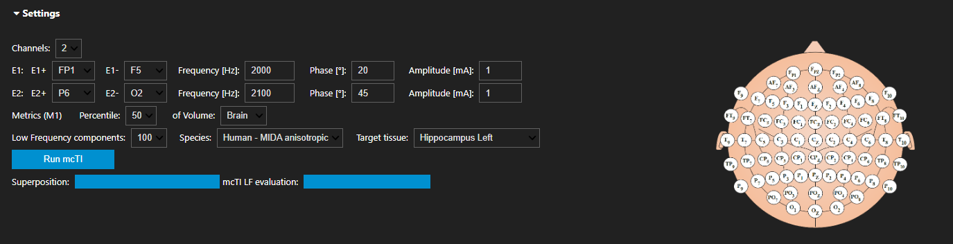
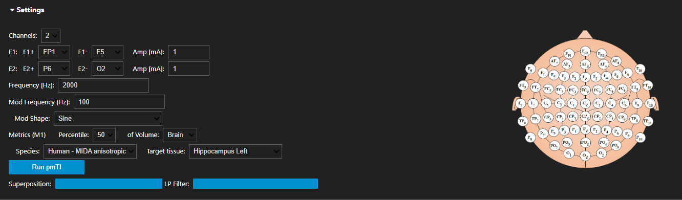
For the non-classic TI modes, the settings are similar, except for the fact that instead of using an automatic optimization, the user defines the setup of interest manually.

Multichannel TI:

Phase-Modulation TI:

Report

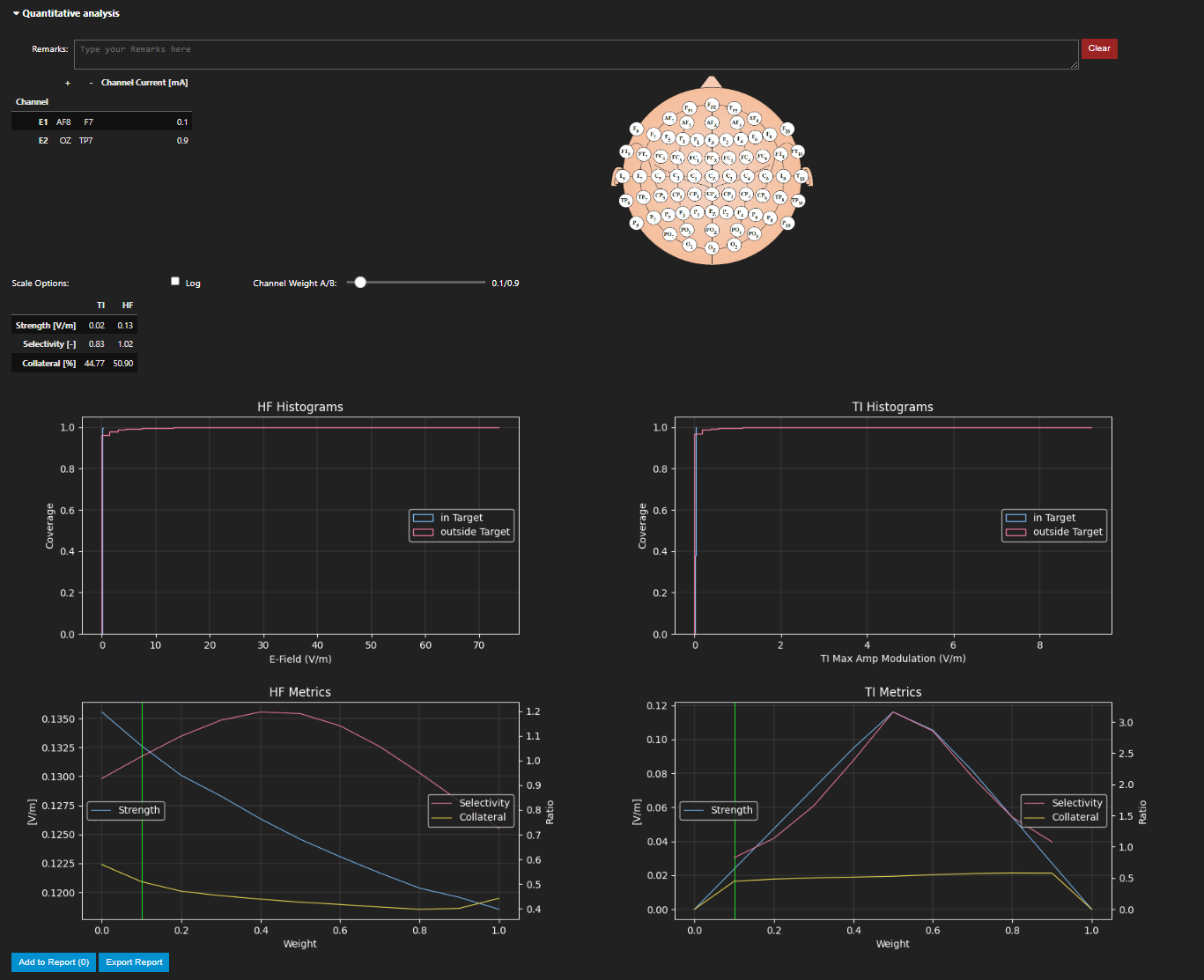
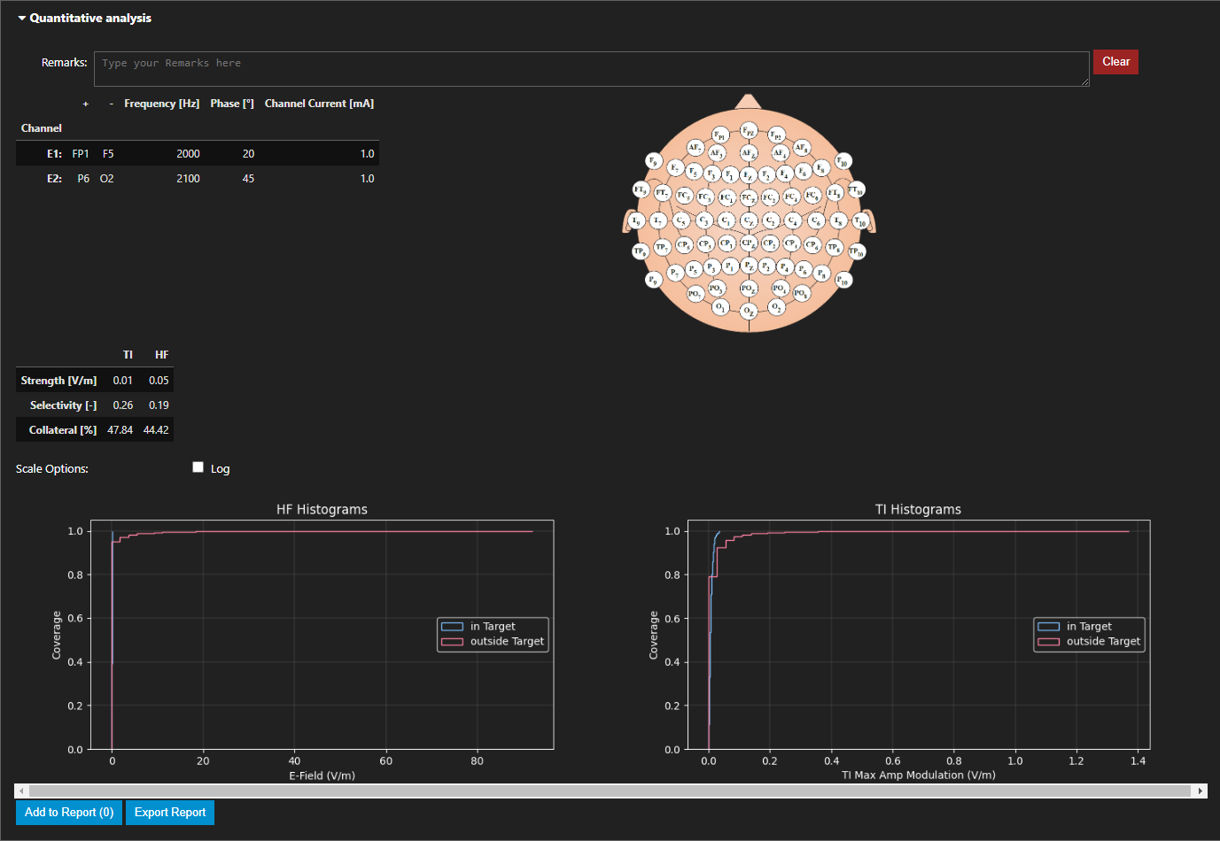
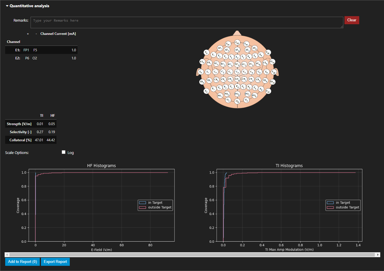
In the Report section, a more detailed and quantitative exposure overview is provided for both high frequency (HF) and temporal interference (TI) fields (compared to the visual one in the Analysis section). A brief explanation of the different parts is as follows:

1. Remarks

   This field can be used to add notes, provide meta-information, and comment. Everything written in this field will be included in the PDF report if this tab is added to the Report by pressing the Add Metrics to Report button.

2. Settings

   Toggle between Log and dB scale and choose the channel weighting.

3. General Information

   The electrode locations, applied currents, and primary metrics for the selected exposure configuration are summarized.

4. Cumulative Histograms

   Cumulative histograms of the HF and TI fields within and outside the target region. Plots for other regions of interest can be added using the dropdown menu.

5. Metrics Plots

   For classic TI, the three principal metrics (Strength, Selectivity, Collateral) are plotted as a function of the channel current ratio (A/B), for both HF and TI fields. This panel is not shown for multi-channel or phase-modulation TI.

6. Export Buttons

   • Add Metrics to Report allows adding all the information from the Report section to the PDF report.
   • Export Report permits the creation and downloading of the PDF report, provided that views, metrics, or curves have been added.